Discretizing ODEs & PDEs: Finite Difference, Finite Element, and Sparse Linear Systems

A story: the first time this clicked for me

The first time I saw a PDE in class, it felt unfair.

The equation was talking about a smooth function $u(x)$ . But my laptop only knows arrays like u[i]. Somewhere in the middle, a professor casually said:

“We discretize the equation and solve a sparse linear system.”

It sounded like a magic spell.

This post is me slowing that spell down until it’s just a series of small, understandable steps—with code you can run and tweak.

The “spell,” expanded

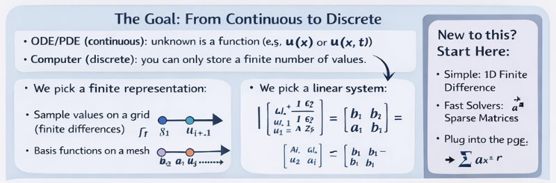
When you discretize, you’re doing three things:

Pick a finite set of unknowns (numbers your computer can store).
Write equations that relate those unknowns (using the physics/math of the ODE/PDE).
Solve the resulting algebra problem (usually $A x = b$ ).

The rest of the story is: how you choose the unknowns (finite difference vs finite element) and how you solve $A x=b$ efficiently (sparse matrices, conditioning, preconditioning, parallelism).

Diagram showing the goal: converting a continuous ODE/PDE into a discrete representation and a linear system Ax=b, with a beginner path: 1D finite difference, sparse solvers, then plug into the PDE. — The core workflow: continuous equation → discrete representation → linear system.

Our tiny test problem (so we can build intuition)

We’ll use a classic 1D problem:

-u''(x) = 1,\quad x\in(0,1),\quad u(0)=u(1)=0

Why this one?

It’s simple enough to implement in one screen of code.
It produces a sparse matrix you can “see.”
It has a known exact solution: $u(x) = \frac{x(1-x)}{2}$ (nice for sanity checks).

Step 1 — Finite difference: turn calculus into a stencil

We’ll create a grid and approximate the second derivative at interior points:

u''(x_i) \approx \frac{u_{i-1}-2u_i+u_{i+1}}{h^2}

Rearranging $-u''(x)=1$ gives a linear equation at each interior point:

\frac{1}{h^2}(-u_{i-1}+2u_i-u_{i+1}) = 1

Stack all those equations together and you get $A x = b$ .

Step 2 — Write it in code (dense first, just to see it)

If you’re learning, it helps to start dense for clarity, then switch to sparse when it makes sense.

import numpy as np

def solve_poisson_1d_dense(n: int):
    # n = number of interior points
    h = 1.0 / (n + 1)
    x = np.linspace(h, 1.0 - h, n)

    A = np.zeros((n, n))
    b = np.ones(n)

    # Tridiagonal: [-1, 2, -1] / h^2
    for i in range(n):
        A[i, i] = 2.0 / (h * h)
        if i - 1 >= 0:
            A[i, i - 1] = -1.0 / (h * h)
        if i + 1 < n:
            A[i, i + 1] = -1.0 / (h * h)

    u = np.linalg.solve(A, b)
    return x, u

At this point, you’ve already “derived a discrete algebraic system.” That’s the core idea.

Step 3 — Notice the pattern: almost everything is zero

Look at A for n=6: only the diagonal and near-diagonals are nonzero.

That is why we use sparse matrices. They store only nonzeros and their indices.

Step 4 — Switch to sparse (the version you actually scale)

Here’s the same thing using SciPy’s sparse tools (CSR under the hood):

import numpy as np
from scipy.sparse import diags
from scipy.sparse.linalg import spsolve

def solve_poisson_1d_sparse(n: int):
    h = 1.0 / (n + 1)
    x = np.linspace(h, 1.0 - h, n)

    main = (2.0 / (h * h)) * np.ones(n)
    off  = (-1.0 / (h * h)) * np.ones(n - 1)

    A = diags([off, main, off], offsets=[-1, 0, 1], format="csr")
    b = np.ones(n)

    u = spsolve(A, b)
    return x, u

Same math. Huge difference in performance and memory once n gets large.

Step 5 — Sanity check against the exact solution

Beginners skip this step and suffer later. Don’t.

import numpy as np

def exact_solution(x):
    return 0.5 * x * (1.0 - x)

def max_error(x, u):
    return np.max(np.abs(u - exact_solution(x)))

If you increase n, the error should go down.

Step 6 — Iterative solvers: how big problems are actually solved

Dense solves and even sparse direct factorization eventually hit memory limits.

For big sparse PDE systems, we usually use iterative methods:

CG (Conjugate Gradient) when $A$ is symmetric positive definite (our case is).
GMRES for more general matrices.

Here’s CG in SciPy:

import numpy as np
from scipy.sparse import diags
from scipy.sparse.linalg import cg, LinearOperator

def solve_poisson_1d_cg(n: int):
    h = 1.0 / (n + 1)
    x = np.linspace(h, 1.0 - h, n)

    main = (2.0 / (h * h)) * np.ones(n)
    off  = (-1.0 / (h * h)) * np.ones(n - 1)
    A = diags([off, main, off], offsets=[-1, 0, 1], format="csr")
    b = np.ones(n)

    u, info = cg(A, b, atol=0, rtol=1e-10, maxiter=5000)
    if info != 0:
        raise RuntimeError(f"CG did not converge (info={info})")
    return x, u

If you try bigger n, CG will still work—but it may take more iterations than you’d like.

Step 7 — The “why won’t this converge?” moment (conditioning)

As you refine the grid (smaller $h$ ), PDE matrices often become more ill-conditioned.

That doesn’t mean your code is wrong. It means your solver needs help.

That help is called preconditioning.

Step 8 — Preconditioning: give CG a better problem to solve

A simple first preconditioner is Jacobi (diagonal scaling). It’s not always the best, but it’s a great learning tool.

import numpy as np
from scipy.sparse import diags
from scipy.sparse.linalg import cg, LinearOperator

def solve_poisson_1d_cg_jacobi(n: int):
    h = 1.0 / (n + 1)
    x = np.linspace(h, 1.0 - h, n)

    main = (2.0 / (h * h)) * np.ones(n)
    off  = (-1.0 / (h * h)) * np.ones(n - 1)
    A = diags([off, main, off], offsets=[-1, 0, 1], format="csr")
    b = np.ones(n)

    inv_diag = 1.0 / A.diagonal()
    M = LinearOperator(A.shape, matvec=lambda v: inv_diag * v)  # M^{-1}v

    u, info = cg(A, b, M=M, atol=0, rtol=1e-10, maxiter=5000)
    if info != 0:
        raise RuntimeError(f"PCG did not converge (info={info})")
    return x, u

On harder problems (2D/3D, variable coefficients), the difference between “no preconditioner” and “good preconditioner” can be the difference between “finishes in seconds” and “never finishes.”

Where finite elements enter the story (intuition first)

Finite difference says:

“My unknowns live on a grid, and derivatives become stencils.”

Finite element says:

“My unknowns are coefficients of basis functions on a mesh, and I assemble contributions element by element.”

You still end up at $A x = b$ . The difference is how you build $A$ and how naturally you can handle geometry/material complexity.

If you want to taste FEM without implementing assembly by hand, tools like FEniCS let you write the math almost directly:

# PSEUDOCODE (FEniCS-style) to show the idea:
#
# mesh = UnitIntervalMesh(n)
# V = FunctionSpace(mesh, "CG", 1)
# u = TrialFunction(V)
# v = TestFunction(V)
# f = Constant(1.0)
#
# a = dot(grad(u), grad(v)) * dx
# L = f * v * dx
#
# bc = DirichletBC(V, Constant(0.0), "on_boundary")
# u_sol = Function(V)
# solve(a == L, u_sol, bc)

Same problem. Different discretization “language.”

The real-world version of this

Once you leave 1D toy problems, your workflow becomes:

discretize (FD/FE/FV) → produce a big sparse $A$ ,
choose an iterative method (CG/GMRES),
choose a preconditioner (ILU, multigrid, domain decomposition),
parallelize (threads/MPI/GPU),
validate (error checks, convergence studies).

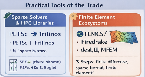
If you want “state-of-the-art” tooling for this:

SciPy is great to learn and prototype.
PETSc/Trilinos are what you graduate into for serious scale and parallelism.

Practical tools of the trade: sparse solvers and HPC libraries (PETSc, Trilinos) and finite element ecosystems (FEniCS, Firedrake, deal.II, MFEM). — A few names worth knowing as you move from learning to real workloads.

A beginner roadmap (hands-on)

Do the dense FD version once so the math feels real.
Switch to sparse CSR (diags, spsolve) and understand why it’s faster.
Try CG and see how iteration counts change with n.
Add Jacobi preconditioning and measure the difference.
Upgrade to 2D (5-point stencil) and feel sparsity/scale.
Then explore FEM (assembly is the big conceptual unlock).

Prerequisites

You’ll move faster if you’re comfortable with:

linear algebra (matrices/vectors; “why $A x=b$ ” is the center)
basic calculus (derivatives, boundary conditions)

If you’ve done linear algebra and the equivalent of MATH/CMPS, you’re set.